


A look at the design concepts used in the application of instrumented systems for safety-related, (protective) functions.
The IEC 61508 standard introduces the concept of functional safety. The standard focuses on deterministic means to define the requirements for protective functions; also deterministic methods to verify the performance of the protective functions. Importantly, functional safety also requires adherence to safety management processes throughout the entire lifecycle in order to reduce systematic failures.
Trip or ESD systems have been around for decades. Originally electrical or electro-mechanical components were used. Over time, these were replaced by programmable logic controllers, (PLCs). This evolution triggered a concern over the integrity of these devices especially the programmability/software aspects. What was needed was a means of quantitatively assessing the system's safety performance.
Characteristics of protective systems
From the analysis phase, all required safeguards would have been defined to address the identified hazards deviations. Some of these safeguards will be implemented using instrumentation, in which case they are called Safety Instrumented Functions, (SIF).
A SIF needs three things:
* A means to detect the occurrence of an unwanted event, (hazard).
* A means to decide what action is needed.
* A means of executing the required action.
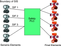
Thus, a SIF may comprise one or more sensing elements, a logic system and one or more final elements. Typically the logic system uses a safety PLC, (alternatively referred to as a logic solver). The term safety instrumented system, (SIS) denotes the complete system incorporating all SIFs required to protect the process plant unit. Normally a single safety PLC is used for the implementation of a SIS, (refer Figure 1).
Although a SIF may look similar to a control system loop, the functional objectives are very different. If a control loop fails, this may well lead to a demand on the SIF. Meanwhile, if the SIF has already failed, then the hazard consequence will result. The SIF must be designed for maximum reliability in order to achieve the safe condition under all operating conditions. Hence a fail-safe circuit is one that assumes the safe state on loss of loop energy.
The perfect SIF is one which is always available to act in the presence of a hazardous condition, (demand) and never causes an unwanted stoppage to plant operation; in essence it never fails.
The financial justification may be shown as follows:
* Failure to act on a process demand = R10M, (once in the lifetime of the system).
* Spurious failures resulting in plant stoppage = R3,75M, (once per year at R250K per incident).
A cost benefit analysis would show that the lifecycle cost of a SIF installed to prevent the above costs presents a positive value. This justification precludes the necessity of protection to personnel and the environment.
Metrics for safety and operational availability
Safety performance could be measured by the extent of the system's availability to perform the safety function when required. However, since safety system performance determination involves the analysis of failure modes, the measurement is expressed as the complement of safety availability ie, safety unavailability, otherwise known as the average probability of failure on demand, (PFDavg). The average value is used due to the time variance of this probability. Figure 2 illustrates the correlation between the process safety requirements: the risk reduction factor, the standardised safety performance unit: safety integrity level, (SIL), safety availability and ultimately safety unavailability or PFDavg.
Operational availability is usually expressed as the spurious trip rate (STR), ie, a frequency rather than probability. Although an approximation, the STR can be viewed as the reciprocal of the mean time to fail safe, (MTTFS). An emergency stop button, if correctly designed, should, under normal conditions have closed contacts and represent a logic one, (healthy) to the safety PLC. If one of the screw terminals becomes loose, an open circuit will exist registering a logic zero, (trip) causing the safety PLC to take the appropriate action: process shutdown.
Overall SIF performance: the weakest link
In the recent past, the focus for safety performance and certification was on the logic solver. Often specifications required TUV certification of this device, however the sensing and final elements were to an extent ignored. With hindsight we now realise that the SIF performance depends on the performance of the entire safety chain. A simple SIF comprising a transmitter, logic solver and valve assembly can be expressed as:
PFDavgsif = PFDavgse +PFDavgls + PFDavgfe
Note that the above expression is an approximation, since the correct formula for logical addition of independent events includes additional terms, however, when dealing with small failure rates (as they should be) the error is normally acceptable as well as being on the conservative side.
What is important is to consider the balance of the contributions to the safety performance from the sensing element, logic solver and final element. It is often the case that one of these components can be responsible for 90% of the overall (lack of) performance of the SIF. Hence the usage of the term: the weakest link.
Safety and reliability
Reliability is key. This requires that the fundamental elements comprising each SIF be designed using high quality components. The design must include strengths that meet or exceed operational stresses, and the installation conditions must be within the design specifications. SIFs are passive since they play no part in active control; therefore testing to ensure that they are still working plays an important role in maintaining integrity. Proof testing involves periodic functionality checks and repair to return the components to the as-new state. The more frequently this is done, the higher the degree of integrity. Automated diagnostic testing extends this concept and greatly improves component safety integrity. The addition of redundancy can improve the component's fault tolerance in respect of PFD and/or STR.
Failure modes and failure rates
Random hardware failures, (as opposed to systematic failures) are generally assumed to be constant over the useful lifetime. As such, the probability of a random hardware failure can be described as an exponential function of time.
Pf(t) = 1 - e-λt
Pf(t): probability of failure
λ : constant failure rate
t : the time variable
It is of importance to distinguish failures that result in the inability of the SIF to perform the safety function, these are called dangerous failures. The complement is known as the safe failure mode that results in a spurious failure. Examining a single component, the total failure rate is expressed as
λ = λs + λd
Where:
λ : total random hardware failure rate,
λs : safe failure rate,
λd : dangerous failure rate.
An example of the different cause and effect failure modes would be a relay used to operate to close a valve during a trip condition. The relay coil is energised and the contacts are closed to apply electrical power to the solenoid valve, which in turn maintains air pressure to the valve actuator to maintain an open position. During the operational period, the relay contacts may become stuck together resulting in the inability to de-energise the loop and close the valve. This then is a dangerous failure. This failure mode is also generally covert, and only becoming apparent in the instance of a demand. An example of a safe failure would be a high resistance forming on the contacts and preventing a closed-circuit loop. The resultant loop de-energisation closes the valve in the absence of a demand. This failure mode is also known as overt, spurious or nuisance due to the consequential disruption to plant operation.
Testing, diagnostics and repair time
The regularity and effectiveness of proof tests improves the probabilistic performance of the SIF. Referring to the probability of failure formula above, if the proof test is assumed to be 100% effective, then the probability of failure on completion of the test returns to the value at installation time. If these tests can be performed automatically and all detected failures either repaired timeously or the affected circuit isolated then the reduction of covert dangerous failures dramatically improves the safety integrity. Examining failure modes again, those failures that are detected are shown as follows:
λ = λsd + λsu + λdd + λdu
where
λ : total random hardware failure rate,
λsd : detected safe failure rate,
λsu : undetected safe failure rate,
λdd : detected dangerous failure rate,
λdu : undetected dangerous failure rate.
A term known as the safe failure fraction describes the degree to which the system is without dangerous undetected failures:
Fault tolerant architectures and common cause
Theoretically, a safety PLC with a low overall reliability, can still achieve a high SFF with the use of diagnostic circuitry. The practical problem here is that diagnostics simply convert the dangerous covert failures into detected failures, which still have to be addressed either by repair or isolation, (shutdown). The net result is a safe system and process plant that is frequently in repair or shutdown.
Redundancy or fault tolerant architectures are used to improve the performance of safety and operational availability. It is however important to distinguish which criterion is to be improved since the choice of architecture may benefit one at the expense of the other. A one-out-of-two, (1oo2) architecture improves safety performance while reducing operational availability, as shown by the example below. A two-out-of-two, (2oo2) architecture has the opposite effect. A two-out-of-three architecture improves both performance criteria, but it comes with a price tag; it is also not much use as a practical valve configuration.
If redundancy is used then the common cause failure mode must be considered. A common cause failure negates or works against the benefits of a fault tolerant architecture since this failure mode has equal influence on all redundant channels. Examples of common cause can include environmental stresses, eg, temperature, EMI, and corrosion. Common cause can also be attributed to software architecture or design, maintenance procedures, design errors and manufacturing problems. The influence of common cause failure mode can be expressed using a beta factor to further categorise failure modes.
λ = βλc + (1-β)λn
where
β : beta factor
The first term denoted λc : failures susceptible to common cause
The second term denoted λn : failures not susceptible to common cause.
The value of beta, (common cause failure) is influenced by the degree of physical separation, electrical separation and diversity among the redundant channels.
Approximation formulas
The influence of the design parameters described above are shown through 1st order approximation formulas as follows:
Case 1: Single channel component with no diagnostics
PFDavg = λd*TI/2
STR = λs
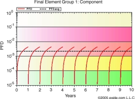
With no fault tolerance and no means to detect unrevealed dangerous failures, the PFDavg is directly proportional to the dangerous failure rate and the proof test period. The STR is simply the safe failure rate.
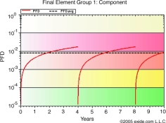
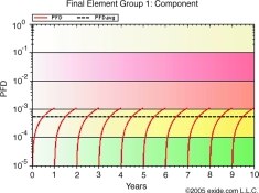
In the example graphs, safe and dangerous failure rates are both equal to 5E-07. In Figure 3, the value of PFD over the mission time of 10 years is shown with a complete proof test occurring every year. In many cases a complete proof test is an invalid assumption, a more likely coverage factor may be 75 to 90%. In this case those dangerous failures not detected during the proof test will remain for the entire operational life of the component. The effect of an incomplete proof test is shown in Figure 4. Figure 5 shows the effect of extending the proof test period. As may be expected, the PFDavg suffers as a result.
Case 2: The effect of diagnostics
PFDavg = λdd*MTTR + λdu*TI/2
STR = (λsd + λsu)
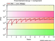
The mean time to restoration, (MTTR) is defined to be the time from failure detection to the time at which repair is complete. PFDavg improves with the degree of failure detection, (diagnostic coverage) and the reduction in the detection and repair time, (normally automated diagnostics are performed within a short cycle time such that the major contribution to the MTTR is in fact the repair time). Figure 6 illustrates the effect of diagnostics on the PFDavg.
Case 3: The effect of fault tolerant architectures
For a one-out-of-two, (1oo2) architecture:
PFDavg =(λd)2 * T2/3
STR = 2λs
The PFDavg is significantly improved since it is the result of the logical AND function of the redundant channels, (both channel 1 and channel 2 must fail in order for the safety function to fail). Note however, that the STR is twice that of the single channel architecture since a safe failure in either will cause a spurious trip.
PFDavg = β(λd*TI/2) + (1-β)(λd*TI)2/3)
STR = βλs + 2(1-β)λs
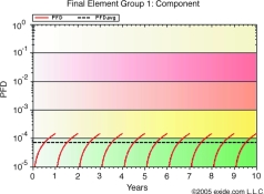
The degree of common cause failure, (beta) has the effect of introducing a single channel component logically ORed with the result of the 1oo2 voting algorithm. The net result is a reduction in the safety performance of the function. Figure 7 illustrates the effect of a 1oo2 fault tolerant architecture.
Component failure data
Determination of the performance of SIFs depends on the availability of accurate failure data for the constituent components. Data collected from operational history and determined using the number of failures divided by the total operational time should be an important source. When using failure data derived in this manner, caution should be exercised due to two factors:
1. Unless great care is taken, equipment failure instances may include systematic failure causes.
2. The service conditions of the equipment should be similar to those expected of the SIF under analysis, alternatively, should be compensation for the service conditions.
Another significant drawback is the lack of failure mode information providing distinction between safe and dangerous failures.
Failure rate data can also be determined quantitatively using a method known as a failure mode effects and diagnostic analysis, (FMEDA). The method is adapted from the better-known FMEA. It is a structured approach that necessitates the analysis of the failure modes, rates and effects of each constituent component of the unit under analysis. The analysis takes consideration of the unit's specification limits and hence provides results that exclude the effects of systematic failure causes. More and more equipment manufacturers are submitting their equipment for independent FMEDA evaluation in the realisation that accurate failure rate information is necessary if the equipment is to be considered for use in safety critical applications.
Architectural constraints
Over and above the PFDavg values calculated by the probabilistic methods described above, the standards place additional constraints on the architectural robustness of each SIF component.
The IEC 61508 bases the constraints on the level of fault tolerance for safety and the degree of absence of undetected dangerous failures, as measured by the safe failure fraction, (SFF). The justification is to provide sufficient architectural robustness and prevent unreasonable claims from failure rates and proof test frequency and adequacy. In this regard IEC 61508 makes a distinction between simple devices and complex devices, the latter generally identified by the level of programmability and degree of uncertainty in the determination of failure effects on the component.
The IEC 61511 has modified the definition of constraints whereby the SFF is replaced by requirements for evidence of reliable performance based on prior use.
Addressing systematic failures
So far the discussions have focused on the effects of random hardware failures on the performance of SIFs. To satisfy the criteria for functional safety, systematic failures must also be addressed. In a survey performed by the Health and Safety Executive, UK, in 1995 involving 34 incidences, 44,1% of the causes were attributed to inadequacies in the control system requirements specification, a further 20,6% were attributed to inadequate management of change, (MOC) procedures. Again, re-emphasising the weakest link phenomenon, the best equipment in existence can be made to malfunction through misuse. The functional safety standards place great emphasis on measures required to manage all activities that can impact on the functionality of the SIF throughout the project and entire operational life. In order to conform to the standards, persons must perform all lifecycle activities with proven competency; also, the progress throughout the lifecycle must include structured verification, validation, and independent audits at specific project milestones.
Conclusion
This article has covered a small part of the lifecycle activities defined by the IEC safety standards. The benefits of the deterministic approach to the quantification of requirements, safety system performance verification and rigorous addressing of the threat of systematic failures are valid reasons for the global acceptance of these standards. Moreover, other sectors, such as manufacturing machinery and nuclear industries are rapidly moving towards harmonisation with IEC 61508.
Advancements have been seen already in the availability of quantified failure data with future trends including the possibility of predicting the influence of environmental stresses on FMEDA produced failure data. Software tools such as SILver are available now, which accurately model the various influences of the parameters discussed in the sections above. The tools themselves require verification by third party certification bodies.
Having the data and the tools are not enough. Functional safety management requires that structures are in place and practised to ensure that all activities throughout the safety lifecycle are conducted with the degree of rigour demanded for the reduction of risk in terms of personnel safety, environmental impact and financial losses as a consequence of out of control processes.
For more information contact Owen Tavener-Smith, Exida, 031 266 8414, [email protected], www.exida.com


© Technews Publishing (Pty) Ltd | All Rights Reserved
 printer friendly version